
Nonlinear Data Assimilation
These pages describe our latest research on data assimilation and a quick guide on what data assimilation is.
Data assimilation combines prior information that we have about a system, e.g. in the form of a model forecast, with observations of that system. It is used in several ways:
- It is a crucial ingredient in weather and ocean forecasting, and is used in all branches of the geosciences. Under different names the method is also used in many othger science disciplines, such as robotics, neurology, biology, traffic control, space weather, cosmology, you name it.
- It is also used to gain better understanding of a system when used in a so-called smoother mode: here we try to find the best description of the evolution of a system over a time window. Studying that description can learn us a lot about the behaviour of the true system, beyond (sparse) observations or a model run alone.
- Finally, it is used heavily in model improvement. The most obvious example is parameter estimation, but more recently we have been pushing parameterization estimation. The latter tries to find a best description of the missing physics in a numerical model, not just the best parameter value. This includes estimating model error covariances.
Typically, the standard data-assimilation methods used in the geosciences look for ‘best estimates’, e.g. the mean or the mode of the posterior probability density. The same tends to be true for so-called inverse problems.
However, present-day problems ask for nonlinear data assimilation in which mean and mode are not enough to describe the posterior probability density satisfactorily. A new paradigm is needed on data asimilation in the geosciences, and that paradigm is there, and already quite old.
It is based on the following observations:
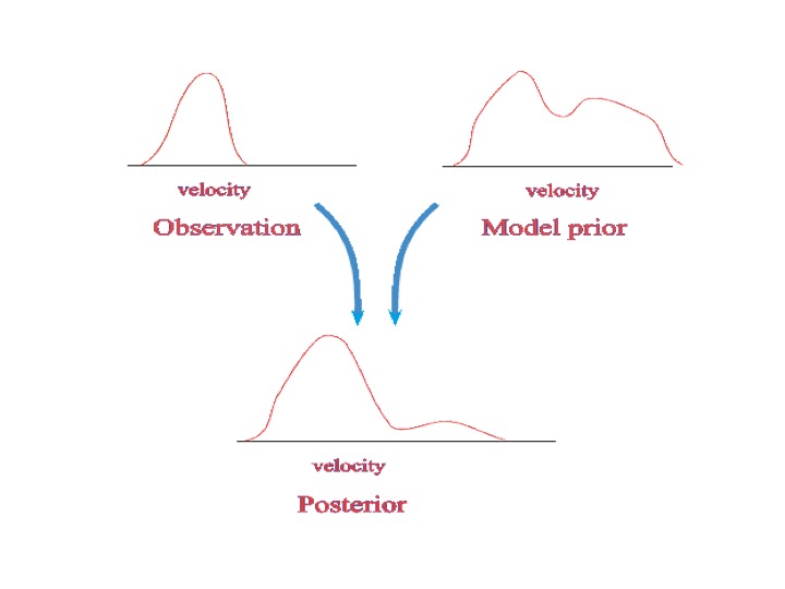
- Data-assimilation and inverse problems can be brought back to Bayes theorem (which can be derived from maximum entropy principles). The general idea is that your knowledge of the system at hand, represented by a probability density function, is updated by observations of the system. The observations are drawn from another known probability density function. Bayes theorem tells us that these two probability densities should be multiplied to find the probability density that describes our updated information
- SO THE SOLUTION TO THE DATA ASSIMILATION PROBLEM IS THIS POSTERIOR PROBABILITY DENSITY FUNCTION, AND DATA ASSIMILATION IS A MULTIPLICATION PROBLEM, NOT AN INVERSE PROBLEM.
- Unfortunately, due to the efficiency of inverse methods for linear Gaussian data-assimilation problems the notion that data assimilation is an inverse problem managed to keep hold of people’s minds. The full nonlinear problem, however, does let us realise that data assimilation is NOT an inverse problem.
- This is true even for parameter estimation. We just have to multiply our prior probability densiity function (pdf) of the parameters with the pdf of the observations (or more accurately, the likelihood, to obtain the updated pdf of the parameters. Really, this is all!!!
This is Bayes Theorem:
(1) 
To exploit this for nonlinear data assimilation we need efficient methods. A possibility is the Particle Filter. Although the standard particle filter is inefficient when a large number of independent observations is assimilated, recent modifications do make particle filters efficient for at least medium dimensional systems (tested even in climate models now), although the solution is not exact anymore. However, Particle Flow Filters turn out to be much more efficient and unbiased even for small ensemble sizes, and we are testing these filters on large to huge dimensional systems right now. Of interest are also techniques from machine learning. While most data-assimilation methods that include machine learning are based on trial and error, and do not generalize well, new developments, such as generative (diffusion-based) machine learning methods are more principled and combining them with e.g. particle flow filters has let to encouraging results.
Our data assimilation research
Our data-assimilation research contains many aspects of the data-assimilation methodology (see also publication list):
- Develop fully nonlinear data assimilation methods, such a particle filters and particle flows, in collaboration with Chih-Chi Hu, Polly Smith, and Manuel Pulido. See our open access recent review in the Quarterly Journal of the Royal Meteorological Society.
- Develop new ways to formulate the data assimilation problem using Ensemble Riemannian Data Assimilation over the Wasserstein Space, with Sagar Tamang and Ardeshir Ebtehaj.
- Infer autoconversion and accretion parameters in cloud systems from LES output and retrieved cloud profiles, in collaboration with Christine Chiu.
- Apply Particle Flow Filters to real-world problems such as understanding the connection between the boundary layer coherent structures and the vortex dynamics in Hurricanes, with Yu-An Chen.
- Apply Particle Flow Filters to understand the drivers of the interocean exchange between the Indian and the South Atlantic Oceans, with Hao-Lun Yeh.
- Apply Ensemble Kalman Filters to hurricanes to understand their rapid intensification phases better. This in collaboration with Michael Bell, Dandan Tao, and Yue (Michael) Ying.
- Develop methods for parameterization and model error estimation, with Magdalena Pulido and Manuel Pulido.
- Understand the behaviour and influence of time-correlated model errors, with Javier Amezcua and Haonan Ren (PhD student).
- Perform Ensemble Kalman Filtering on Arctic sea ice over a 25-year period to better understand the sea-ice retreat of the last decade, with Nick Williams (PhD student), Danny Feltham, Ross Bannister, and Maria Broadridge.
- Investigate mergers between Machine Learning and Data Assimilation. This is work with Manuel Pulido and Chih-Chi Hu.
- Research on better understanding of Ensemble Kalman Filters
- Efficient minimization techniques, saddle point formulations, ensembles of vars, with Amos Lawless, Jennifer Scott and Ieva Dauzickaite (PhD student)
- Efficient data-assimilation methods for space weather and solar physics
Particle filters
In Particle filtering the prior probability density function (pdf) is represented by a set of particles, or ensemble members, each equal to a possible state drawn from the prior pdf. This set of particles is propagated with the full nonlinear model equatiuons to the next observation time. There the particles are compared to the observations, and the closer the particle is to all observations (defined by the value of the likelihood of that particle) the higher its weight. The result of this is a set of weighted particles. These weighted particles now represent the posterior pdf. The following figure demonstrates the procedure:
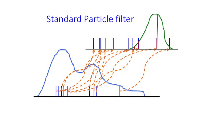
Standard Particle Filter. The blue curve denotes the prior pdf at the start of the data-assimilation experiment, from which the particles (blue vertical bars) are drawn. The size of the bar is the weight of the particle. These particles are then propagated by the model equation to the next observation time (orange dashed lines). At observation time they appear as the blue bars, representing the prior at that time. The likelihood of the observations is given by the green curve. Now we have to apply Bayes Theorem, so we multipli the blue bars by the green curve values, leading to the red bars. These red bars represent the posterior pdf. Note that that representation is rather poor, only one or two particles get a high weight, while the rest gets a weights very close to zero. We need more sophisticated particle filters than this method…
We have been working hard to develop more efficient particle filters than the above Standard Particle Filter. An example are so-called Equal-Weight Particle Filters, which instead of just weighting the particles move them around in state space such that they all obtain equal weight. This is an example of a Proposal Density Particle Filter. We have applied these particle filters to many systems, including a climate model. For a recent review see this open access paper.
Recently we managed to find interesting refinements of the equal-qeight particle filters that explore synchronization, and other methods that remove the bias typically present in these methods. Parallel to this we investigate so-called particle flows.
Particle Flows
Particle flows are a special kind of particle filters in which the particles are not weighted at observation time, but instead moved around in state space via an ordinary differential equation in pseudo time. Remember that this pseudo-time evolution happens all at observation time! The following two figures illustrate the methodology. This is a very exciting field and new results will be added soon. See our most recent open access paper.
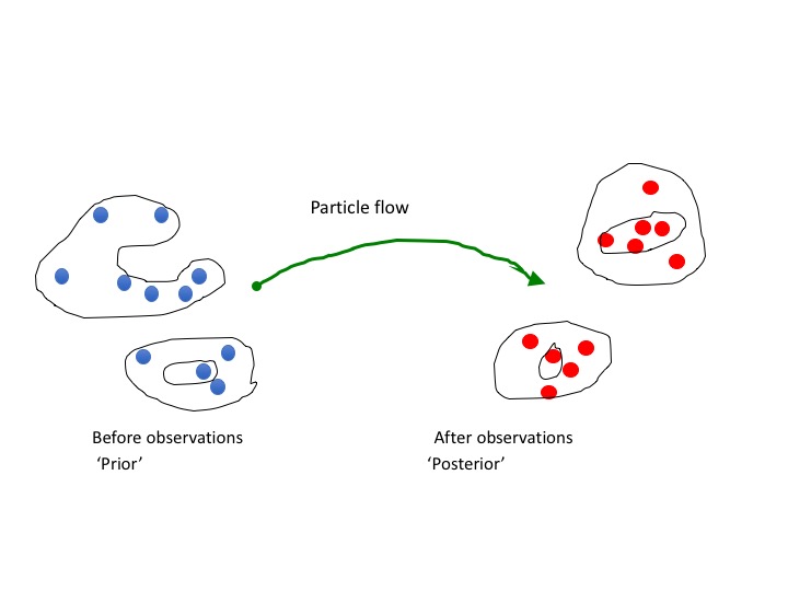
Illustration of a particle flow. At each observation time we smoothly move the prior particles (so samples from the prior) to samples from the posterior by solving a differential equation in psuedo time.
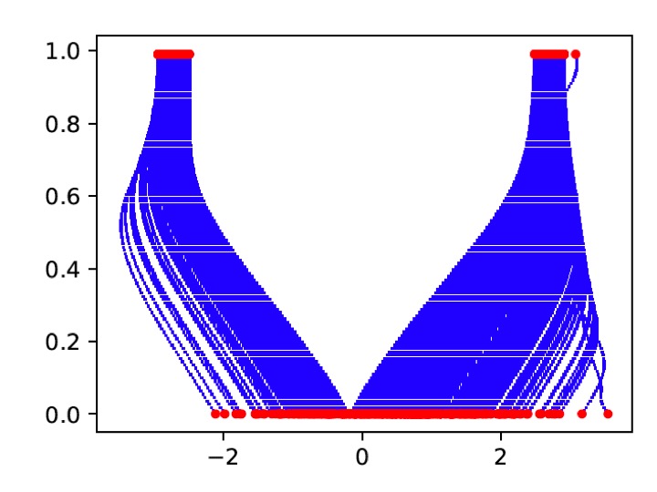
Example of a 1-dimensional particle flow. The horizontal axis is the value of the state, the verticle axis pseudo time. The red dots at the bottom are the prior particle positions, the blue lines their evolution in psuedo time, and the red dots at the top are the posterior particle positions.